BiasPruner: Debiased Continual Learning for Medical Image Classification

Continual Learning (CL) is pivotal for enabling neural networks to adapt dynamically by learning tasks sequentially without forgetting prior knowledge. However, traditional CL methods often overlook a critical challenge: the existence and transfer of dataset biases, particularly in sensitive domains like medical imaging. These biases can lead to shortcut learning, compromising generalization and fairness. Addressing this gap, BiasPruner introduces a novel approach by intentionally forgetting spurious correlations. By leveraging a bias score to identify and prune biased units, BiasPruner forms task-specific debiased subnetworks, preserved for future use. Experiments on medical datasets demonstrate BiasPruner’s superior performance in accuracy and fairness, advancing CL solutions.

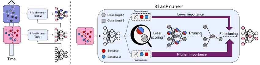
BiasPruner employs a fixed-size network f capable of learning an unknown number of tasks (T) sequentially without catastrophic forgetting. During the training of the t-th task, the network exclusively processes biased training data D_t=(x_i,y_i) where y_i∈C_t and the set of classes (C_t​) may vary with each task, including new classes.

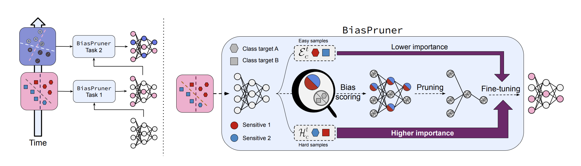
BiasPruner consists of three main components: Bias Scoring, Bias-aware Pruning and Finetuning, and Task-agnostic Inference.

Bias Scoring: Identifying Spurious Features

Bias scoring is the process of quantifying how much each unit in a network contributes to shortcut learning caused by spurious correlations in the training data. This process involves three critical steps: Training the model to be biased, Partitioning the training data, and Calculating bias scores for network units.

Step 1: Train the Model to Be Biased and Learn Spurious Features

To detect spurious features, the network is deliberately trained to fit biased data using the Generalized Cross Entropy (GCE) loss:

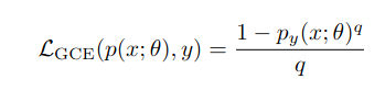
where

• p(x;θ): Softmax output of the network.
• p_y(x;θ): Probability assigned to the correct class y.
• q ∈ (0,1]: Hyperparameter controlling bias amplification.

Compared to the cross-entropy (CE) loss, the GCE loss prioritizes "easier" samples by up-weighting the gradient for high-confidence predictions

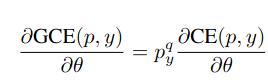
In this paper, the authors assume that the easier samples contain the spirious features. Therefore, by focusing on these easier samples, the network becomes biased, learning shortcuts and spurious correlations instead of generalizable patterns.

Step 2: Partitioning the Training Data

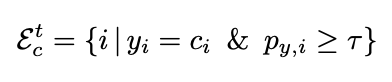
After training the biased model, the training dataset {x,y} is divided into biased and unbiased sample sets for each class c:

• Easy Sample Set (E_t,c): consists of samples correctly classified by the network with high confidence

• Hard Sample Set (H_t,c): consists of samples misclassified by the network, even with high confidence.

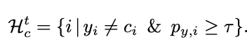
This partitioning isolates biased examples (easy to learn due to spurious correlations) from unbiased ones (harder to learn and generalizable).

Step 3: Bias Scoring for Network Units

To quantify the contribution of each unit nnn to shortcut learning, a bias score is calculated based on the unit’s activation variance for biased and unbiased samples. For a given class ccc, the bias score for unit n is calculated as:

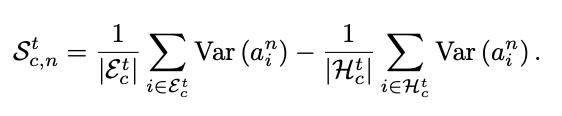
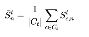
Var(a_n,i) represents the variance of the feature map a_n,i over its spatial dimensions (w, h). Units that respond more strongly to biased samples than to unbiased samples are assigned higher bias scores, designating them as the main contributors to learning shortcuts in the network. The final bias score for unit nnn is averaged over all classes:

Bias-aware Pruning and Finetuning

To ensure fairness and generalization, BiasPruner removes biased units and fine-tunes the network. Units with the highest bias scores (top γ%) are pruned, including their filters and feature maps. This pruning step removes reliance on shortcuts and forms a task-specific debiased subnetwork (f_t​).

After pruning, the subnetwork is fine-tuned with a Weighted Cross Entropy Loss (L_WCE) to recover performance and prioritize hard-to-learn samples. The loss function is defined as:

α ∈ (0, 1) is a trainable parameter, and L_GCE(x) is the sample’s GCE loss value of the biased networks obtained while scoring bias. By this loss function, easy samples (small L_GCE(x)) are down-weighted while hard samples (large L_GCE(x)) are up-weighted exponentially.

While finetuning this subnetworks, all the units associated with the subnetworks from the previous tasks are frozen to avoid forgetting the previously acquired knowledge.

Task-agnostic Inference

Task-agnostic inference in BiasPruner enables the model to handle scenarios where the task identity of a test image is unknown. Using a maxoutput strategy, BiasPruner identifies the most relevant task-specific subnetwork by evaluating the maximum output response across all subnetworks for a given test batch. Specifically, the task t^∗ is selected as:

where ϕ_t represents the fully connected layer and θ_t the parameters of the t-th subnetwork. Once t^∗ is identified, BiasPruner uses the subnetwork f_t^* to make predictions:

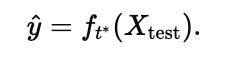
This ensures accurate classification without requiring explicit task labels, making BiasPruner dynamic, scalable, and practical for real-world continual learning applications.

Experiments and Results

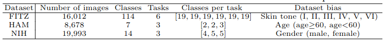
The effectiveness of BiasPruner was evaluated across three datasets—Fitzpatrick17K (FITZ), HAM10000 (HAM), and NIH ChestX-Ray14 (NIH)—chosen for their dataset biases, class variety, and public availability. Each dataset was divided into non-overlapping tasks, with FITZ, HAM, and NIH split into 6, 3, and 3 tasks, respectively.

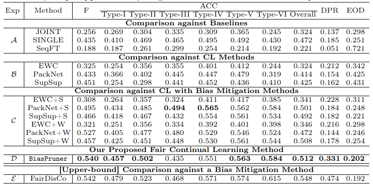
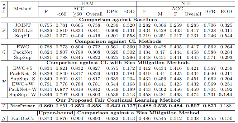
Evaluation Metrics included accuracy metrics like F1-score (F) and balanced accuracy (ACC), as well as fairness metrics like Demographic Parity Ratio (DPR) and Equal Opportunity Difference (EOD). Results were averaged across all tasks at the end of learning.

Using ResNet-50 as the backbone, BiasPruner was trained with GCE loss (q=0.7) for 200 epochs, pruning 60% of biased units, and fine-tuning with LWCE for 20 epochs.

Results:

• Compared to baselines like JOINT, SINGLE, and SeqFT, BiasPruner significantly improved fairness and accuracy. SINGLE showed better fairness than JOINT but suffered from catastrophic forgetting.
• On FITZ dataset, against other CL methods like EWC, PackNet, and SupSup, BiasPruner outperformed in fairness , as these methods did not address dataset bias.
• On age- and gender-biased datasets, BiasPruner consistently outperformed baselines and debiasing-enhanced methods in both classification and fairness metrics.
• Even after enhancing baselines with debiasing algorithms (e.g., resampling and reweighting), they fell short of BiasPruner's performance.
• BiasPruner achieved performance comparable to FairDisCo, a bias-mitigation method using explicit bias annotations, despite not using such annotations.

Conclusion

BiasPruner is a novel continual learning framework that improves fairness and mitigates catastrophic forgetting through intentional forgetting. By identifying and pruning network units responsible for spurious feature learning, BiasPruner constructs debiased subnetworks for each task. Experiments on three datasets show that BiasPruner consistently outperforms baseline and CL methods in both classification performance and fairness. However, the paper has some limitations: it does not address the time complexity of the method, it does not explore the potential reappearance of shortcuts (bias) after pruning and fine-tuning, and it assumes that bias is always easier to learn, which may not hold in all scenarios. These results emphasize the importance of addressing dataset bias in future continual learning approaches.

References

1. Nourhan Bayasi, Jamil Fayyad, Alceu Bissoto, Ghassan Hamarneh, Rafeef Garbi BiasPruner: Debiased Continual Learning for Medical Image Classification. https://arxiv.org/pdf/2305.08396
2. Nam, J., Cha, H., Ahn, S., Lee, J., Shin, J.: Learning from failure: De-biasing classifier from biased classifier. Advances in Neural Information Processing Systems 33, 20673–20684 (2020). https://arxiv.org/pdf/2007.02561