Computed tomography scan

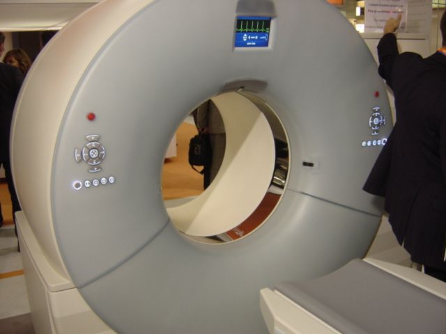
Principle of scanner aquisition

We have an object or a human being and want to get information about its inside structure. A scanner will do the following steps to measure such information:

• Select a layer/plane, moving a motorized table.
• Select a line in the plane, moving an X-ray source.
• Send a ray (a monochromatic x-ray) following the line.
• Measure the ray's intensity after it crossed the object
• Compute the quotient of the measured intensity by the emmited intensity
• Store the result
• Repeat the process for many lines.
• Repeat for many parallel planes.

Attenuation rate

The data aquired by a scanner contains a lot of information, however, not directly interpretable by a doctor. We need information about each point. Here we have information related to the attenuation of a line that crossed the body. In order to transform the raw data to human-readable data, our first goal is to understand precisely the scanner raw data.

The attenuation equation allows to measure how much a ray of light is reduced when it crosses an object

I_r = I_eexp(-∫_Lf(x)dx)

Where:
• I_r is the emmited intensity of the ray.
• I_e is the recived intensity of the ray.
• L is the line of the ray.
• f is the attenuation function of the object.

The goal of a CT scanner is to compute the function f. It gives a lot of information about the body. Various tissues have different attenuation rates for x-ray.

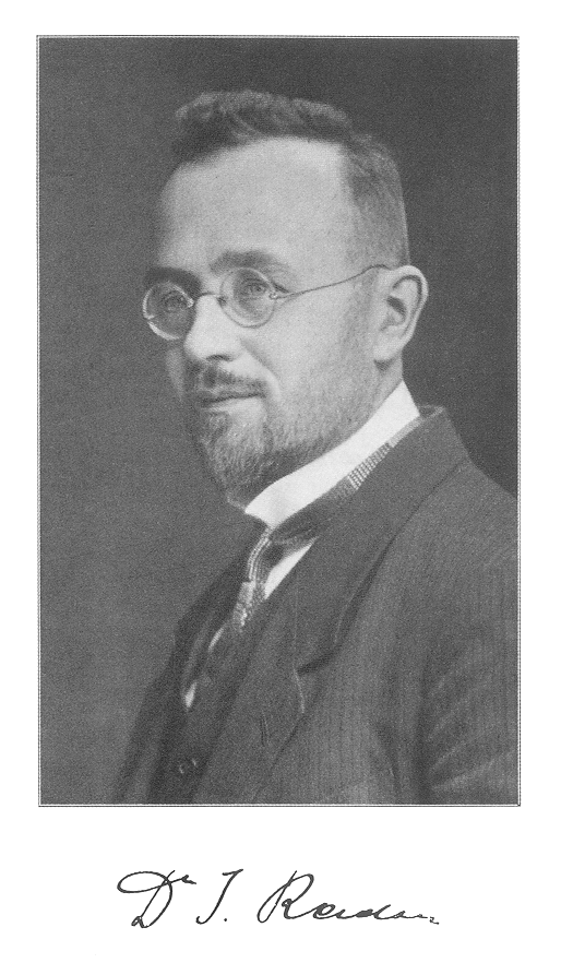
The Radon's transform of a function

Johann Radon was an Austrian mathematician, he defined a transformation on functions in 1917. This transform is now named Radon in his honor. Moreover, Radon proved that his transformation is invertible. One can compute back the original function from its transform.

Let f: ℝ²→ℝ be a function. The Radon's transform of f is a function defined on the set of all lines, by the following formula for a line L.

$R$f(L) = ∫_Lf(x)dx

Observe that up to $-log$ a scanner measures the Radon transform of our function of interest f. In order to complete a CT Scan we only need to inverse the Radon transform, which was done by Radon a century ago.

Polar parametrisation for lines

The Radon's transform of a function is defined on the set of all lines, which is not convenient for representation, as this set might be hard to visualize. However, for each line we can associate a real number ρ and an angle α in [0,π] which uniquely represent the line.

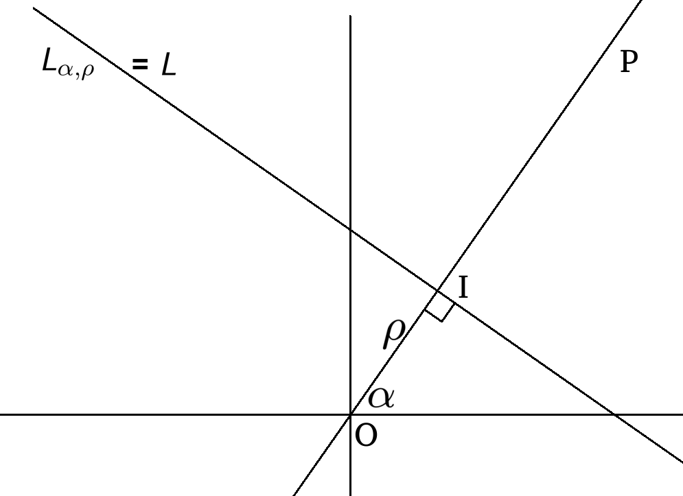
Consider a line L, denoted by P the line that goes through the origin O and is orthogonal to L. Let I be the intersection of P and L. We set ρ to be the measure of OI (positive if I is in the upper half-plane and negative if I is in the lower half-plane). Moreover α is the (line) angle that forms between the L and P. Reversing the construction, we can define L_ρ,α=L.

The points of the line L_ρ,α=L can be parametrized by the real numbers using the following formula:

L_ρ,α(t) = (ρcosα-tsinα, ρsinα+tcosα)

We can rewrite the formula for the Radon's transform of f.

Rf(ρ,α) = ∫_ℝf(ρcosα-tsinα, ρsinα+tcosα)dt

This formula allows to display Radon's transform as images, indeed by taking the angle α on the horizontal axis and distance ρ on the vertical axis, we associate numbers to points of the planes, which defines an image.

We show above a circle and its Radon's transform. Observe that the columns of the Radon transform are all the same. Indeed due to the rotational symmetry of the circle, the integral does not depend on the angle, but only on the distance to the origin.

Inverse Radon's transform

Using several transforms, including Fourier's direct and inverse transform, Radon, was able to find an algorithm to compute the inverse of Radon's transform. This result remains dormant for over fifty years before it was first used for inverting scanner acquisition, and so obtaining the attenuation rate of an object.